달리는 말킹

Task5 Perform a principal components analysis

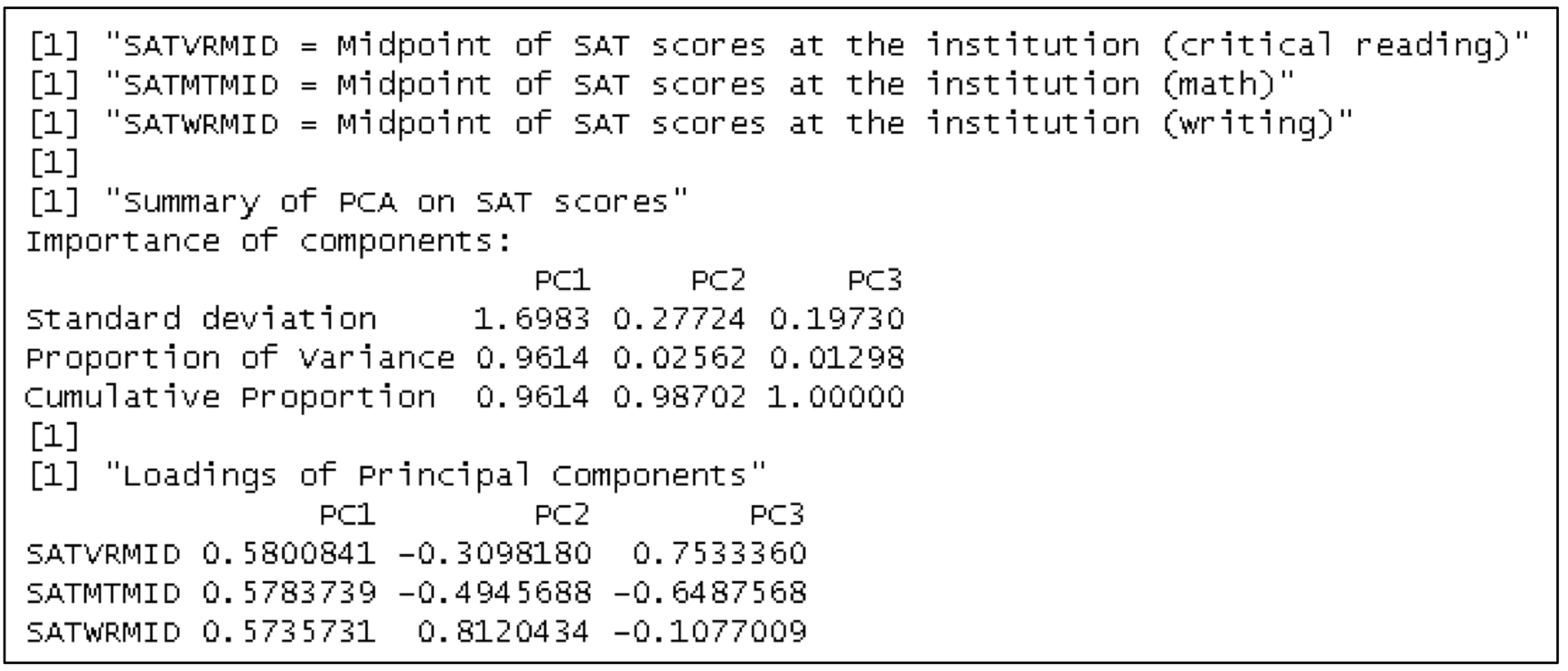
  Principal components analysis is a method to summarize high dimensional numeric data with fewer dimensions while preserving the spread of the data. It can be particularly helpful when variables are highly correlated. PCA finds orthogonal linear combinations of the input variables (which are typically centered and scaled) called principal components (PCs) that maximize variance to retain as much information as possible. The principal components are ordered according to their variance. The sum of their variances is the total variance explained. It is then common to look at the proportion of variance explained by each principal component to decide how many PCs to use.

 Advantages

 PCA could allow us to build a simpler model with fewer features. PCA can help visualize high-dimensional data to explore relationships between variables. PCA can help identify latent variables.

 Disadvantages

 Using a subset of the principal components results in some information loss. The principal components will be less interpretable than the original variable inputs. Although PCA reduces dimensionality in the model, the original variables must still be collected for future predictions, so no efficiency is obtained.

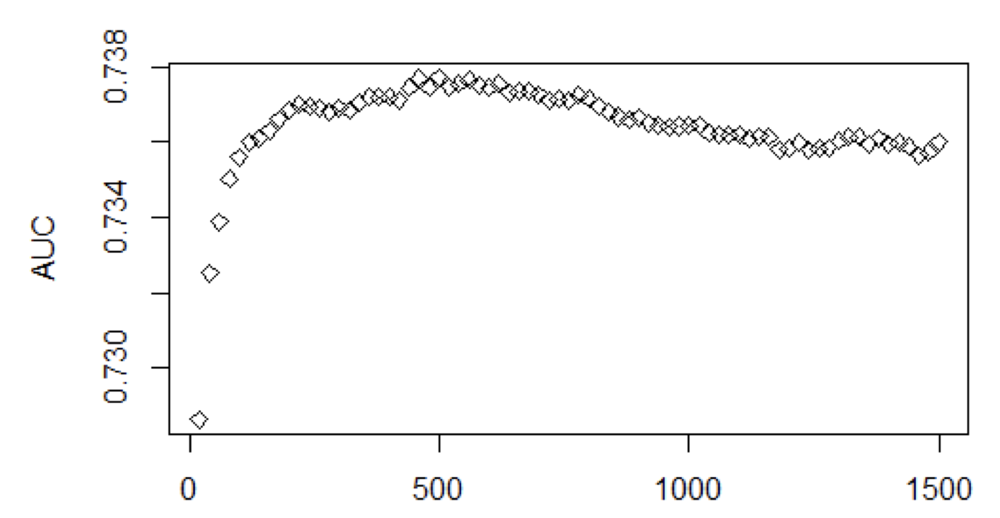
Task6 Construct a decision tree

  When a decision tree is trained, it can become very large and include splits that are not particularly valuable for predictions on new data. When examining the fit of a tree, it is a good idea to try to prune a tree when it has many splits that do not improve performance. Pruning reduces the size of the tree, hopefully removing less valuable splits from the tree. This process reduces overfitting the tree on the training data, can lead to better predictions, and results in a simpler, more interpretable tree.

Task9 Discuss the bias-variance tradeoff

 Bias is the expected loss caused by the model not being complex enough to capture the signal in the data. Variance is the expected loss from the model being too complex and overfitting to the training data.

 With high variance (overfitting), the model will perform better on the training set than on a test set. With high bias (underfitting), the model will perform poorly on both the training set and the test set.

Task2 Construct a classification tree

 Split the data in to training(70%) and testing (30%) sets.

 Alter the minbucket, cp, maxdepth parameters. Each of these parameters can be used to prevent overfitting. The "minbucket" parameter sets the smallest size for any leaf node in the tree. The "cp" paramter sets the minimum improvement needed in order to make a split. The "maxdepth" parameter sets the minimum number of levels for the splits.

 Estimate the cp parameter using cross-validation. Dividing the training data up into folds, training the model on all but one of the folds, and measuring the performance on the remaining fold. This process is repeated to develop a distribution of performance values for a given cp value. The cp value that yields the best accuracy is then selected.

Task3 Construct a random forest

 Generally, variables that are used to make splits more frequently and earlier in the trees in the random forest are determined to be more important.

Task4  Consider a boosted tree

  Random forests use bagging to produce many independent trees. When a split is to be considered, only a randomly selected subset of variables is considered. each tree is built from a bootstrap sample from the data. This approach is designed to reduce overfitting, which is likely when a single tree is used.

 Boosted trees are built sequentially. A first tree is built in the usual way. Then another tree is fit to the residuals (errors) and is added to the first tree. This allows the second tree to focus on observations on which the first tree performed poorly. Additional trees are then added with cross-validation used to decide when to stop (and prevent overfitting).

 Both random forests and boosted trees are ensemble methods, which means that rather than creating a single tree, many trees are produced. Neither method is transparent, so they require variable importance measures to understand the extent to which input variable is used.

 Random forests do not use the residuals to build successive trees, so there is less risk of overfitting as a result of building too many trees, while boosted trees will result in a lower bias. The best boosted trees learn slowly (use lots of trees) and thus can take longer than a random forest to train.

Task5 k-means clustering

 The goal is to assign records into one of k groups or clusters such that members of each group are overall more similar to one another than they are to menbers of other groups. The numbers of groups, k, is specified at the beginning and the group members are determined through an iterative process. k random centers are chosen and the group assignment for each record is determined by which of these centers is closest. New centers for each group are calculated based on its members, and then group membership is redetermined based on these new centers. This process continues until the centers and group membership are stable or stopped by an interation limit.

Task7 Boosting

 Boosting builds up an ensembel model, taking the aggregate prediction of many individual models or learners, each successive model building on the deficiencies of the prior model. Unlike bagging, another ensemble method, the individual models are not independent. The technique gains accuracy not by the particular predictions of any of its individual models, often called weak learners, but by its iterative process for improving the aggregate performance of the models in total.

 The first model is trained on unweighted data, and then second model is trained on the residuals produced by the first model. The thired model is trained based on the residuals of the first two models taken together, and so on. The boosting process is typically stopped after a set number of iterations, and the sum of all model output is used.

 To prevent overfitting within this terative process, a shrinkage parameter is applied to individual models so that the aggregate performance of the models approaches the training data in a controlled manner and avoids being overly sensitive to the structure of any one model.

 Boosting is appropriate for this business problem because its predictions, by directly addressing the errors of prior model fittings, are typically more accurate than those of other predictive modeling techniques. Being a more complex ensemble method, it is difficult to gather insight into how the model is making these accurate predictions, but this seems relatively unimportant to ABC.

 Partial dependence plots use the expected value of the prediction at the variable value shown when paired with all values of the other variables as found in the training data. The yhat values can be compared to the overall average mean bike usage of 189 per hour in the train data.

 The higher shrinkage parameter, representing greater weight for each weak learner, produces a substantially better prediction as measured by mean squared error. The higher shrinkage get faster without overfitting. Because the higher shrinkage parameter gives more weight to each model fitting the successive residuals, the predictions tend to be more spread out given the same number of trees.

https://eatchu.tistory.com/entry/앙상블Ensemble-bias-variance-관점에서의-유형-정리-Voting-Bagging-Boosting

네이버에서 검색한 블로그인데 유튜브에서 찾은 것들보다 설명이 잘되어있다. (블로그 주인님께 감사드림...)

Task8 Compare disitribution choices for a glm

 Poisson distribution with log link function is a reasonable choice. The target varaible only has non-negative integer values. The log link function allows the predicted mean to vary multiplicatively rather than linearly with the coefficients for each predictor variable, more naturally fitting the right-skewed distribution of the targer variable.

 The gamma distribution with inverse link function is also a reasonable choice. There is not material harm in applying the gamma distribution function to only integer values when the values span a large range. The data matches its support of strictly non-negative values, though it is conceivable that future data could include zero bike rentals. The inverse link function allows the predicted mean to vary hyperbolically rather than linearly with the coefficients for each predictor variable. Unlike the log link function, the inverse link function can result in nagative predictions, typically massive and unusable when they occur.

Task6

(a) Explain what the variance and bias values indicate about the relative quality of predictions when comparing predictive models.

 The variance figures indicate how much the predictions vary depending on the training data used. As more predictors are used, the variance increases because the model more predicsely fits the training data for each trial and becomes less generalized. The bias figures indicate how close expected predictions and actual results are on unseen data. Generally, as more predictors are used, the bias decreases as more accurate predictions are made.

Task7

(a) Explain, for a general audience, what cost complexity pruining does.

 Cost complexity pruninig is part of a two-step approach to building a tree model. The first step is to build a large, complex decision tree, which is essentially a flow chart for deciding whether to try to transfer an animal.

 A second step called pruning is taken. Pruning reduces the size and complexity of the initial flow chart to a more useful one. That is is called cost complexity pruning has to do with the technical tradeoff being made between how simple the flow chart is compared to how well it distinguishes whether animals can be transferred or not.

Task8

(a) Boosting - Setting eta as high as possible?

 In boosting algorithms, which work by iteratively fitting a model the residuals of a prior learner, eta, also called the learning rate or shrinkage parameter, slows down the model fitting process so that the residuals from the prior learner do not have too large an influence on the final model. With eta at its maximum of 1, each model iteration is the prior learner plus the model fitting its residuals. While this will run quickly, it will be prone to high variance, overfitting the training data and not generalizing well to unseen data. Setting eta to less than 1 slows down the fitting process by only adding eta times the model fitting the residuals to form the next learner and will substantially reduce the variance.

(b) Explain cross validation and how it can be used to set the eta hyperparameter

 Cross validation divides the availabel data in to multiple folds for a series of model fitting runs. Each fold is used as test data exactly once. The average test metric across the runs is the result of the cross validation.

 To use cross validation to set the eta hyperparameter, a series of reasonable values for eta would be chosen beforehand. Then, for each value of eta, cross validation would be performed with each model fitting run using the same eta. The result is one average test metric result from each cross validation for each value of eta. The value of eta with the superior test metric, some measure of predictive power on unseen data, would be shosen for subsequent predictive modeling work.

Task6

(a) GLM, each of the Gaussian, Poisson and Gamma distribution.

 Gaussian

 - The domain is all real values.

 - A target variable that could be modeled with the Gaussian distribution is the response time.

 Poisson

 - The domain is non-negative integers.

 - A target variable that could be modeled with the Poisson distribution is the number of calls in an hour.

 Gamma distribution

 - The domain is positive real values.

 - A target variable that could be modeled with the Gamma distribution is the turnout time plus one second since it is continuous and postive.

Task9

(a) Explain how measures of impurity are related to information gain in a decision tree

 Information gain is the decrease in impurity created by a decision tree split. At each node of the decision tree, the model selects the split that results in the most information gain. Therefore, the choice of impurity measure(e.g, Gini or entropy) directly impacts information gain calculations.

(c) When concerned about the model variance, Recommend whether to use a random forest or a gradient boosting machine.

 I recommend a random forest, which tends to do well in reducing variance while having a similar bias to that of a basic tree model. The variance reduction arises from the use of many small trees and sampling of the data (bagging). Both practices hinder overfitting to the idiosyncrsies of the training data, and hence keep the variance low.

 Gradient boosting machines use the same underlying training data at each step. This is very effective at reducing bias but is very sensitive to the training data(high variance)

Task10

(a) explain why decision trees overfit to factor variables with many levels.

In this task, the number of levels is 31. This means the number of ways to split day of the month in to two groups is very large, making it likely that the tree will find spurious splits that happens to produce information gain for that particular training data.

 Decision trees tend to create splits on categorical variables with many levels because it is easier to choose a split where the inofrmation gain is large. However, splitting on these variables will likely to lead to overfitting.

(b) Describe the handling of categorical variables in linear models and tree-based models.

 Linear Models : 

 The coefficients for each level represents the impact relative to the base level of the variable.

 Tree-Based Models : 

 The more levels the variable has, the more potential ways to split the category into groups. split based on maximizing information gain. Decision trees naturally allow for interactions between categorical variables based on how the tree is created.

Task11

(c) Explain what let to the large difference in AUC values between the train and test datasets.

 An AUC of 1.0 indicates the model perfectly predicts the data while an AUC of 0.5 indicates the model performs as well as random chance.

 This indecates that the models are overfit to noise in the training datasets. The likely cause is that the chosen hyperparameters create very deep trees, and therefore the hyperparameters need to be adjusted to create simpler trees which are less prone to overfitting.

Task13

(a) Explain how cost-complexity pruning works, including how complexity is optimized.

 Cost-complexity pruning involves growing a large tree and then pruning it back by dropping splits that do not reduce the model error by a fixed value determined by the complexity parameter. We can use cross validation to optimize the complexity parameter, which is the process repeatedly training models and testing models on different folds of the data. This is done for different values for the complexity parameter, and the one with the lowest cross validation error is selected as the optimal choice. We then prune back our trained tree using the complexity parameter from the cross validation.

(b) State why changing the random seed would affect the tree constructed using cost-complexity pruning.

 Each time the cost-complexity pruning algorithm is run, the splits of data used in the cross validation are randomly assigned.

Task8

(a) cost-complexity pruning algorithm

 Pruning is a technique used to reduce the complexity of a decision tree and protect against overfitting. This process is repeated for each remaining split until further pruning would result in decreased model accuracy.

https://www.youtube.com/watch?v=D0efHEJsfHo

(b) Choosing a complexity parameter based on cross-validation results.

 Choosing the value that results in the minimum corss-validation error.

 Employing the one standard-error rule. This approachproposes using the complexity parameter for the smallest model within one standard-error of the minimum cross-validation error.

Task9

(a) Explain the difference between accuracy and AUC in terms of overall model assessment.

 Accuracy is measured by the ratio of correct number of predictions to total number of predictions made.

 AUC measures the area under the ROC curve. It assesses the overall model performance by measuring how true positive rate and false positive rate trade off across a range of possible classification thresholds.

 AUC measures performance across the full range of thresholds while accuracy measures performance only at the selected threshold.

(b) Explain why the ROC curve always goes through (0,0) and (1,1)

(0,0) : true positive rate(Sensitivity) is zero, and true negative rate(Specificity) is 1.

(1,1) : true positive rate(Sensitivity) is 1, and true negative rate(Specificity) is zero. everything is classified as postiive.

https://www.youtube.com/watch?v=4jRBRDbJemM

(c) Gradient boosting machine tree model, Explain why model performance deteriorates as the number of trees increases.

A GBM iteratively builds trees fit to the residuals of prior trees. Depending on the hyperparameters, this model can produce a very complex model, which is susceptible to overfitting to patterns in the training data.

 AUC on the testing data starts to drop, which indecates the model is overfit to the training data.

https://www.youtube.com/watch?v=LsK-xG1cLYA

https://www.youtube.com/watch?v=3CC4N4z3GJc

https://www.youtube.com/watch?v=2xudPOBz-vs

 잘 이해 안된다.  틈틈히 다시보자.

(d)  Describe two hyperparameters to improve model performance.

 Early stopping : Early stopping criteria, such as improvement of the performance metrics in each subsequent tree, can stop training when it detects the improvement is marginal. This avoids overfitting.

 Controlling learning rate : Learning rate controls the impact of subsequent trees to the overall model outcome. This reduces the extent to which a single tree is able to influence the model fitting process.

(e) How to tune a hyperparameter.

 Tuning a hyperparamether requires first varying the hyperparameter across a range of possible values and performing cross validation at each value. Performance is then determined based on a cross-validation performance metric, for example AUC, and the hyperparameter value with best performance based on this metric is selected.

Task11

(d) How changing the link function in the GLM impacts the model fitting and how this can impact predictor significance.

 The link function specifies a functional relationship between the linear predictor and the mean of the distribution of the outcome conditional on the predictor variables. Different link functions have different shapes and can therefore fit to different nolinear relationships between the predictors and the target variable.

 When the link function matches the relationship of a predictor variable, the mean of the outcome distribution (the prediction) will generally be close to the actual values for the target variable, resulting in smaller residuals and more significant p-values.

Task12

(a) Proxy variable

 Proxy variables are variables that are used in place of other information, usually because the desired information is either impossible or impractical to measure. For a variable to be a good proxy it must have a close relationship with the variable of interest.

Task2

(c) Discuss the benefits of stratified sampling

 Stratified sampling results in test and train datasets that are similar with respect to the stratification variables. 

Wikipedia

In statistics, stratified sampling is a method of sampling from a population which can be partitioned into subpopulations.

In computational statistics, stratified sampling is a method of variance reduction when Monte Carlo methods are used to estimate population statistics from a known population.[1]

Task3

(c) best subset selection vs stepwise selection

 best subset selection > global minimum

 stepwise selection > local minimum, computationally more efficient

> 시험장가서 각 기법 설명를 영어로 할수 있을지 모르겠다 ㅋ

Task4

(a) Describe two ways impurity measures are used in a classification tree.

 - which split in the decision tree should be made next.

 - which branches of the tree to prune back after building a decision tree.

https://www.youtube.com/watch?v=_L39rN6gz7Y&t=348s

Task5

(a) Poisson regression vs Quasi-Poisson regression

 An underlying assumption of Poisson regression is that the mean and variance are equal.

 Quasi-Poisson regression is equipped to deal with the problem of overdispersion. the estimates of the coefficients are the same when compared to the Poisson output. However, the standard errors are all higher and fewer coefficients are statistically significant. If any further analysis is conducted such as deriving confidence intervals or conducting hypothesis tests, the quasi-Poisson distribution should be used.

Task8

(a) Compare and contrast stepwise selection with shrinkage methods.

Similarities

 - both avoid overfitting to the data, especially when the number of observations is small compared to the number of predictors.

 - both can be used for variable selection to reduce model complexity.

Differences

 - Stepwise selection takes iterative steps, until there is no improvements as measured by AIC.

 - Shrinkage methods can reduce the size of coefficients without entirely eliminating variables.

(b) Explain why variables are standardized as part of the lasso model fitting procedure.

 Variables that are on a larger scale typically have smaller coefficients and vice-versa. Without standardizing, the regularization will focus on shrinking the variables on a smaller scale over those on a larger scale.

(c) Describe the process of searching for the optimal value of the hyperparameter lambda in a lasso regression.

 The optimal value for lambda can be found using cross-validation. First, a grid of lambda values is chosen for the search. Then for each lambda value, a cross-validation error is calculated.

 The first step in calculating a cross-validation error is to partition the data into k folds. A single fold is removed for testing, and the remaining folds are used to train a lasso model with the current lambda value. This process is prepeated for each of the k partition, and a cross-validation error is calculated as the average of an error measure (e.g. RMSE or AUC) across all k testing partitions.

 The optimal lambda value is the one with the lowest cross-validation error.

https://www.youtube.com/watch?v=fSytzGwwBVw

cross validation statQuest에도 있는데 이주제는 ISLR책이 더 잘 이해되는거 같음.

(f) confusion matrix

sensitivity = TP/(TP+FN)

specificity = TN/(TN+FP)

https://www.youtube.com/watch?v=vP06aMoz4v8

텍스트로 볼때는 와닿지 않았는데 영상으로 보니 언제 sensitivity나 specificity가 높은걸 써야하는지 알수 있었음. 3개, 4개의 경우도.

(g) lowering the cutoff threshold?

 Assess the consequences of this recommendation as it relates to the business problem.

 This will increase positive predictions (both TP and FP) while reducing negative predictions (both TN and FN), increasing sensitivity. 

Task9

(a) Describe how baagging is used in the random forest algorithm and the advantage it gives random forests over a single decision tree in terms of the bias/variance trade-off

 Random forests are created by applying bagging and taking random feature subsets to construct multiple trees, which are averaged to produce a prediction.

 Bagging is the process of training of multiple models in parallel on different random subsets of the data. Each individual tree is trained on a different training dataset. Variance refers to the sensitivity of the model to changes in the training dataset. Bagging reduces variance because each individual tree is trained on different data.

Task2

(a) Explain how PCA is typically used.

 PCA is an unsupervised learing techniqque that creates new uncorrelated variables that mazimize variance. Often, the first few principal components explain most of the variability in the original variables. These principal components can be used in place of the original variables to reduce dimensionality and create a simpler model.

(b) PCA 특징

 PCA is effective when there is high dimensionality (many variables) which can make univariate and bivariate data exploration and visualization techniques less effective. PCA is used to summarize high-dimensional data into fewer composite variables while retaining as much information as possible.

 PCA attempts to maximize the variance or spread in our data distribution by linearly combining original variables.

Task3

(a) assumptions for OLS

 - The residuals have a normal distribution.

 - The mean of the residual is zero.

 - The residual variance is constant.(homoscedasticity)

Task4 ridge/lasso/elastic net

(b) 

> ridge/lasso/elastic-net 주제도 뭔가 텍스트로 보면 잘 와닿지 않은데 StatQuest에서 시각화 잘해서 알려준다...

overfitting 방지하기 위한 방법론이다, ridge vs lasso 차이(coefficient 0 가능한지) 이상의 문제가 나오면 대응 가능할지 모르겠다. 

https://www.youtube.com/watch?v=Q81RR3yKn30

https://www.youtube.com/watch?v=NGf0voTMlcs

https://www.youtube.com/watch?v=Xm2C_gTAl8c

https://www.youtube.com/watch?v=1dKRdX9bfIo

Task8

(a) Interpret standard daeviation and proportion of variance in the output.

 A standard deviation of 1.6983 implies strong correlation among the three SAT features.

 The proportion of variance 0.9614(PC1) implies that the three SAT variables are highly correltated and that it is reasonable to use PC1 as a replacement for the three SAT scores a predictive model.

(b) Interpret the "Loadings of Principal Components" for PC1 and PC2

 The similar loading values in PC1 implies that the SAT scores in three-dimensional space fall near the line Writing SAT = Math SAT = Reading SAT. PC1 primarily prepresents the average score because PC1 is correlated with the direction of any of the SAT variables.

 PC2 shows that the residual variance not explained by PC1 can be mostly explained by the Reading SAT and the Math SAT being positively correlated with each other and negatively correlated with the Writing SAT.(흠?)

https://www.youtube.com/watch?v=FgakZw6K1QQ

 설명변수가 많아질때 차원줄이는 방법론이다 보니 글로 봐선 직관적으로 이해 안됬는데 시각화해서 잘 설명해주는 듯.

https://www.youtube.com/watch?v=HMOI_lkzW08

 위 영상보다 컴팩트한 버젼! 뭐있나해서 봤는데 위에꺼 봤으면 아래꺼 안봐도 되긴할듯.

Task10

(a) Explain why tree-based models are resilient to outliers in predictor variables.

 By partitioning the outliers, their effect can be isolated from the other leaves, resulting in the body of the distribution being unaffectied.

(b) Recommend which metric to use for outliers in the target variable. RMSE vs MAE

 I recommend MAE because it is more robust to outliers. Outliers tend to result in large error terms, which have an outsized impact on RMSE, due to the squaring of the error term.